

Price impact is structural to AMMs
Constant-product AMMs usex · y = k to price trades against pool reserves. A trade changes the reserve ratio, so larger trades move further along the curve. This is how the AMM works, not a defect in the design.
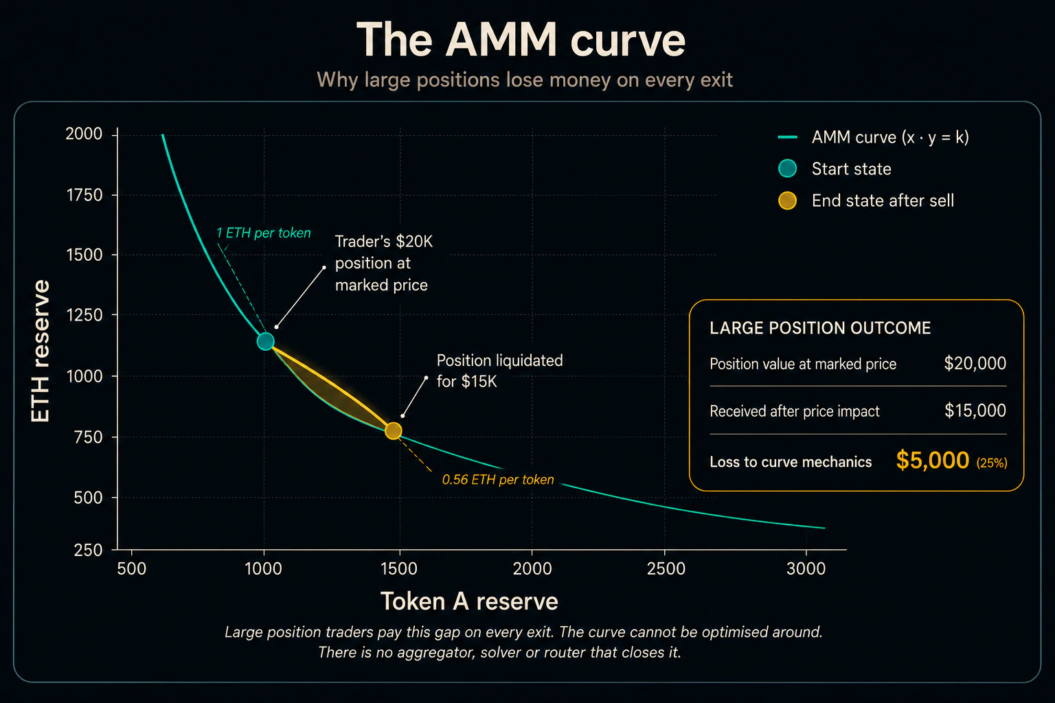
Illustrative constant-product price impact as trade size grows
This table is a mathematical illustration of a basic constant-product pool, not a prediction for a routed trade. Real execution depends on fees, concentrated liquidity, route splitting, market movement and depth across venues.
Routing can find liquidity. It cannot manufacture it
Aggregators and solvers improve execution by searching across available venues. They can split routes, compare prices and use alternative liquidity sources. What they cannot do is remove the structural price impact of a liquidity source that is too shallow for the requested size. If every available route ultimately relies on limited curve-based depth, better routing can reduce the problem without eliminating the underlying constraint. That creates a gap between two things that are often treated as the same decision:- Immediate market execution: cross the liquidity that exists now and accept the resulting executable price.
- Making inventory available: expose a position to market demand and allow it to be consumed as buyers arrive.
Where concentrated inventory comes from
Thin-liquidity markets regularly accumulate sell-side inventory from:- project and foundation treasuries
- funds and venture investors
- founder, team and advisor allocations
- unlock and distribution events
- market makers and professional traders
- whales and other concentrated holders
- platforms that originate or control eligible inventory flows
The missing liquidity layer
C1 Pools introduce a separate inventory source alongside existing AMM, RFQ, order-book and intent liquidity. The C1 execution rate is derived from an oracle rather than from the pool’s reserve balance. A C1 fill therefore has no C1 pool-induced price impact. The broader market price can still move, execution can still fail if protection conditions are not met and deposited inventory is not guaranteed to fill immediately. The key change is structural: the seller can place inventory into a shared liquidity layer and let existing buyer demand consume it progressively through integrated execution infrastructure.Market scope
FlowState is designed for trades where order size is material relative to available AMM liquidity, particularly where conventional AMM execution would result in more than 1% price impact relative to the pre-trade reference price. Rather than defining this opportunity with a fixed annual trading-volume estimate, FlowState treats it as an execution condition. The amount of flow that meets that condition changes with market volume, liquidity depth and the routes available at the time of execution.Next: C1 Pools Explained
How FlowState turns single-sided token inventory into a liquidity source for existing market demand.